Example: TD-CDFT for MoS2 Monolayer (NewResponse)

Download NewResp_2DMoS2Restart.run

This example demonstrates how to calculate the frequency-dependent dielectric function with the help of the NewResponse implementation for a two-dimensional system. (see NewResponse) Furthermore, the general setup to run the TD-CDFT section as a restart calculation is presented as well. This allows for splitting of the frequency range into several parts, which can then be calculated in separate calculation without the overhead of evaluating the groundstate properties for each of them! Hence, it is a trivial parallelization possibility.

Groundstate Optimization

$ADFBIN/band <<EOF
  GeometryFile MoS2_2D_1L.xyz

  Symmetry NoSym

  NumericalQuality basic
  Relativistic ZORA

  KSpace
    Grid 5 5
  End

  BasisDefaults
    BasisType DZP
    Core      Large
  End

  End input
EOF
mv RUNKF restart.runkf

TD-CDFT+Restart Calculation

Caution

One has to make sure to use the same Symmetry/NumericalQuality/KSpace/BasisDefaults/ZORA/... options for the groundstate calculation and for the restart calculation! Otherwise a normal groundstate SCF optimization will be performed in the restart calculation.

$ADFBIN/band <<EOF
  GeometryFile MoS2_2D_1L.xyz

  Symmetry NoSym

  NumericalQuality basic
  Relativistic ZORA

  KSpace
    Grid 5 5
  End

  BasisDefaults
    BasisType DZP
    Core      Large
  End

  Restart
    SCF
    File restart.runkf
  End

  NewResponse
    nFreq        11
    FreqLow      2.0
    FreqHigh     3.0
    ActiveESpace 10.0
  End

  NewResponseSCF
    nCycle       30
  End

  End input
EOF
mv RUNKF prop.runkf

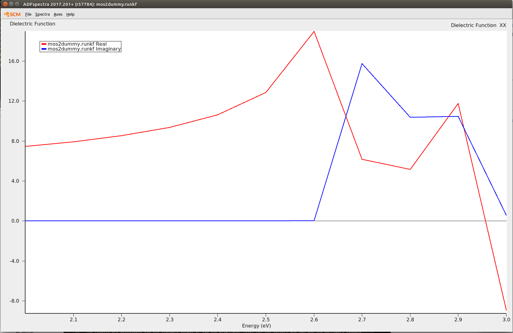
The results are accessible via the standard output or via the prop.runkf file. For the latter, one can use the ADFreport command $ADFBIN/adfreport prop.runkf RESPDIELRE and $ADFBIN/adfreport prop.runkf RESPDIELIM to print the components of the dielectric function for the real (RESPDIELRE) and imaginary (RESPDIELIM) part separately. In the following tables, only the diagonal components are presented:

Real part

Frequency (au)	\(\epsilon_1(XX)\)	\(\epsilon_1(YY)\)	\(\epsilon_1(ZZ)\)
0.0735	8.1622063	8.1788067	1.8845925
0.0772	8.7718566	8.7960299	1.8891231
0.0808	9.6251443	9.6631930	1.8941277
0.0845	10.9457271	11.0126367	1.8996502
0.0882	13.4618956	13.6001321	1.9057858
0.0919	26.5135344	25.9300685	1.9126665
0.0955	6.1134118	4.1756368	1.9204849
0.0992	6.2789015	4.6880515	1.9295347
0.1029	13.7665058	11.5484340	1.9403044
0.1066	-7.2575153	-5.8285172	1.9537079
0.1102	-0.7937277	1.2661253	1.9718981

Imaginary part

Frequency (au)	\(\epsilon_2(XX)\)	\(\epsilon_2(YY)\)	\(\epsilon_2(ZZ)\)
0.0735	0.0015601	0.0015758	0.0000213
0.0772	0.0020566	0.0020839	0.0000200
0.0808	0.0029274	0.0029798	0.0000216
0.0845	0.0047632	0.0048794	0.0000231
0.0882	0.0104743	0.0107877	0.0000246
0.0919	0.2658531	0.1942899	0.0000264
0.0955	12.8856772	14.5286319	0.0000294
0.0992	9.7571573	10.1567455	0.0000338
0.1029	7.5936072	6.7674596	0.0000399
0.1066	13.0264038	9.5897946	0.0000487
0.1102	0.2483041	0.3222301	0.0000676

The more convenient option is to plot the spectral data directly with the help of ADFspectra. Just type:

$ADFBIN/adfspectra prop.runkf