Calculating sigma profiles with all models
This example demonstrates how to calculate COSMO-RS sigma profiles with both available models (SG1 and FS1). We’ll use 4-Methylphenol for this example. The variable ref_sp in the script is the \(\sigma\)-profile calculated in the AMS COSMO-RS.
import pyCRS
import matplotlib.pyplot as plt
chdens = [-0.025 + 0.001*x for x in range(51)]
ref_sp = [0.00000000, 0.00000000, 0.00000000, 0.00000000, 0.00000000, 0.17050209, 0.73517288, 0.98383886, 0.86397332, 1.15571158, 0.67051286, 0.79380670, 0.71422825, 0.68854784, 0.72126747, 0.72414167, 0.83293801, 2.33617486, 5.42197092, 8.58230745, 9.84294559, 8.81993395, 8.80932110, 6.79578176, 6.57764296, 6.07802490, 9.19651976, 11.04721719, 12.80255519, 11.17672544, 12.28788009, 10.72121222, 2.77829981, 1.11136819, 1.58235813, 1.13444125, 1.81316980, 2.44468560, 2.02558727, 0.01243933, 0.00000000, 0.00000000, 0.00000000, 0.00000000, 0.00000000, 0.00000000, 0.00000000, 0.00000000, 0.00000000, 0.00000000, 0.00000000]
mol = pyCRS.Input.read_smiles("Cc1ccc(O)cc1")
pyCRS.FastSigma.estimate(mol,method="COSMO-RS",model="FS1")
sp_fs1 = mol.get_sigma_profile()['Total Profile']
pyCRS.FastSigma.estimate(mol,method="COSMO-RS",model="SG1")
sp_sg1 = mol.get_sigma_profile()['Total Profile']
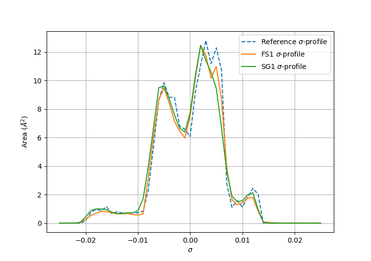
plt.plot(chdens, ref_sp, '--', label="Reference $\sigma$-profile")
plt.plot(chdens, sp_fs1, label="FS1 $\sigma$-profile")
plt.plot(chdens, sp_sg1, label="SG1 $\sigma$-profile")
plt.ylabel("Area ($\AA^2$)")
plt.xlabel("$\sigma$")
plt.grid()
plt.legend()
plt.show()
Finally, the plot produced shows the various \(\sigma\)-profiles produced.