Viscosity of an ionic liquid with APPLE&P
In this tutorial we will describe how to compute the viscosity of an electrolyte mixture using the APPLE&P polarizable force-field. We will take as an example the mixture of N-methyl-N-butylpyrrolidinium (pyr14) and bis(trifluoromethane sulfone imide) (TFSI) (1:1 ratio).
Important
This tutorial requires AMS2023 or later.
Note
In order to extract a reliable value for the viscosity the system must be well equilibrated. The short equilibration times proposed in this tutorial are only provided to enable the calculations on a desktop computer however, a realistic example would make use of a Linux cluster.
Warning
In this tutorial, the Python snippets are only here to illustrate some important PLAMS commands to reproduce the GUI settings and are not meant to be executed. An example of the integration of these PLAMS commands in consistent program is provided in the optional Python workflow below.
Optional: Download a PLAMS Python workflow to run the entire MD simulations described
below with a single command.
Creating the system
Let’s start by creating the atomic structure with the Builder.
PYR14 = from_smiles("CCCC[N+]1(CCCC1)C")
TFSI = from_smiles("C(F)(F)(F)S(=O)(=O)[N-]S(=O)(=O)C(F)(F)F")

box = appleandp_packmol(
    molecules=[PYR14, TFSI],
    n_molecules=[30, 30],
    density=0.5,
    region_names=["cation", "anion"],
    forcefield_file=forcefield_file
)
Note
The special function appleandp_packmol is a combination of packmol to fill the simulation box with a given set of molecules, and APPLE&P atomtyping (that generates the force field file named PYR14_TFSI.ff).
Note
The density provided is in g/cm3.
We intentionally chose not to fill the box to the experimental density of 1367 kg/m3, we will adjust the density later.
Setting up the calculation
Next we need to set up the APPLE&P engine.
s = Settings()
s.input.ForceField.Type = 'APPLE&P'
s.input.ForceField.ForceFieldFile = os.path.abspath(forcefield_file)
Note
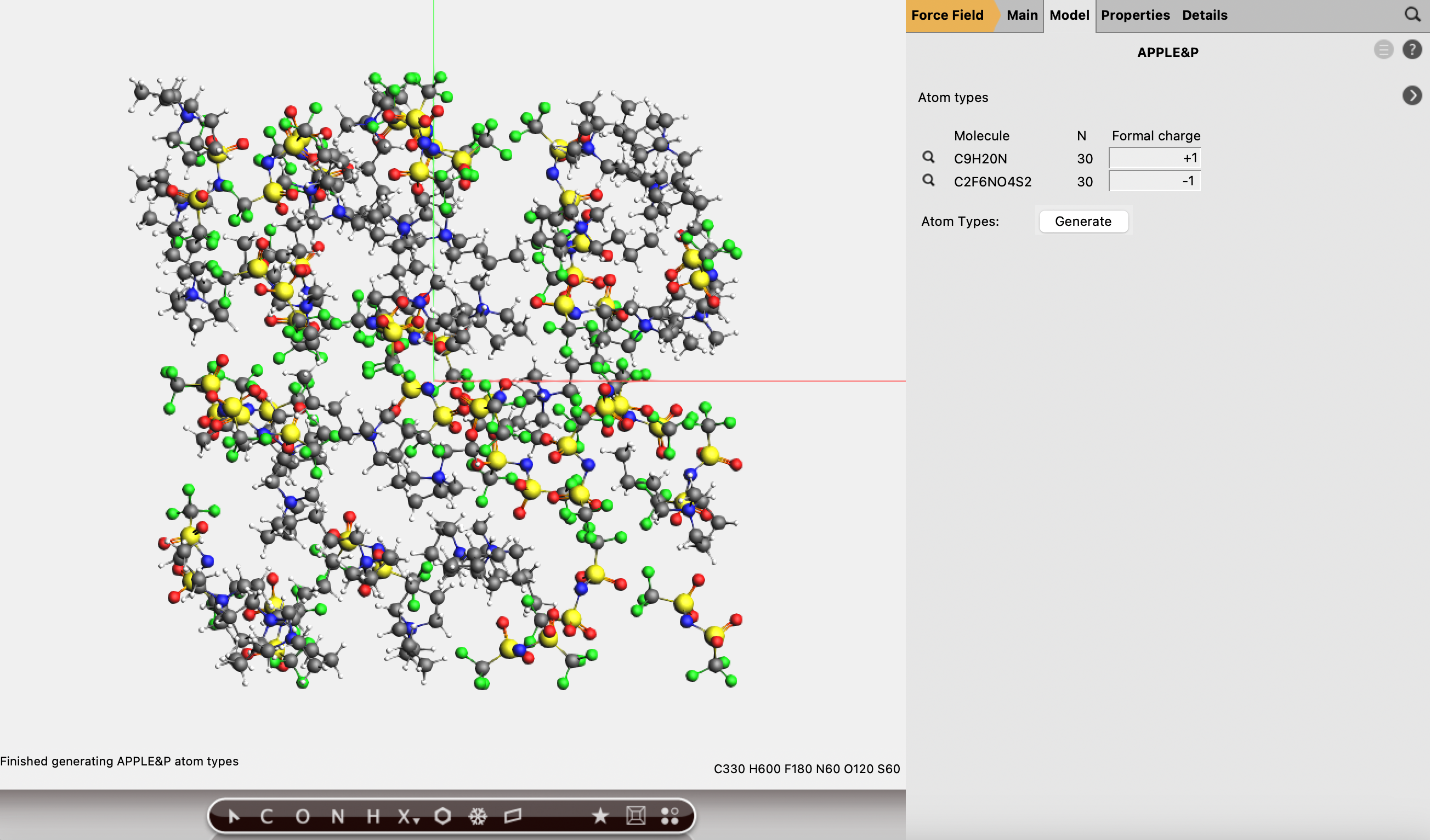
When you click to generate, the APPLE&P tool will perform a connectivity analysis and identify the atom type of each element in the system. The tool will then write a force field in your working directory with the extension .ff.
Note
If you enter incorrect charges, AMSinput will display an error message. You can also see that the parameters are all set when you see the message Finished generating APPLE&P atom types in the bottom-left corner of the molecule panel.
Pre-optimization
It’s always a good idea to perform a quick optimization of the system.
From the Main tab.
s_preopt = Settings()
s_preopt.input.ams.task = 'GeometryOptimization'
s_preopt.input.ams.GeometryOptimization.MaxIterations = 10
s_preopt.input.ams.GeometryOptimization.PretendConverged = 'Yes'
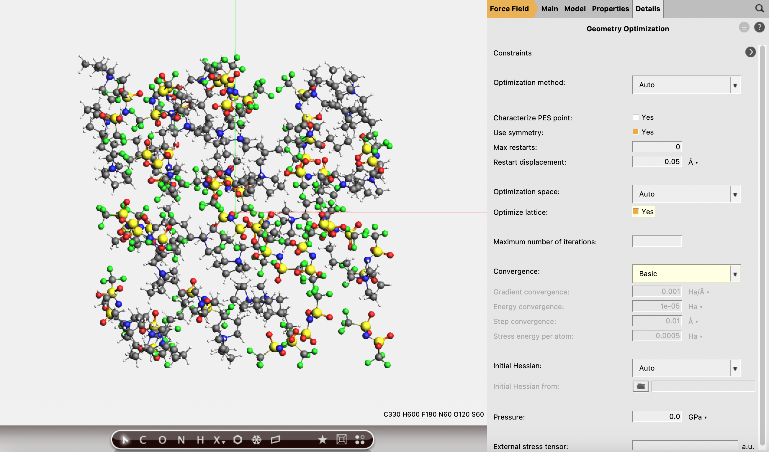
You can now save the input as appViscosity_preopt (for example), and run the pre-optimization.
Adjusting the simulation box
We would like now to adjust the simulation box dimensions in order to obtain a density close to the experimental density of 1367 kg/m3. Click View → Properties to display various information about the system. The current density is approximately 491 kg/m3. In order to reach a reasonable density, we need to shrink the simulation box. We will therefore perform molecular dynamics under deformation to reduce the simulation box dimensions to the target size. Let’s first define the MD settings:
Note
With APPLE&P it is recommended to use a timestep smaller than 1 fs.
We now define the deformations. The deformation procedure will linearly adjust the simulation box to the target dimension during the molecular dynamics simulation. A bit of algebra gives us the equation for the final cell dimension \(L_{f} = \sqrt[3]{\frac{\rho_i}{\rho_f}}L_i \approx 25\) Å.
Note
We do not need to be very precise in the final volume as we will later perform an isobaric simulation and let the density of the system equilibrate.
Note
If you previously performed the pre-optimization with Python, you would like to import the final molecule to pass the ScanDensity job. This can be achieved as follow:
mol = job.results.get_main_molecule()
job = AMSMDScanDensityJob(
    scan_density_upper=1.36,
    molecule=mol,
    settings=s,
    name="scan_density",
    nsteps=10000,
    timestep=0.5,
    temperature=333,
    writevelocities=False,
    writemolecules=False,
    writebonds=False,
)
Save your calculation as appViscosity_scandensity, and run it. It should take about 10 minutes on a modern laptop. Click yes when asked to update the coordinates. You can appreciate the volume change from SCM → Movie. You can check that the density of the system is now close to the experimental value from View → Properties.
Thermalization
We will now perform a short molecular dynamics simulation in the canonical ensemble (NVT) at 333 K to thermalize the system.
job = AMSNVTJob.restart_from(
    job,
    settings=s,
    name="NVT_before_NPT",
    nsteps=10000,
    timestep=0.5,
    temperature=333,
    writevelocities=False,
    writemolecules=False,
    writebonds=False,
)
Note
Here we use the AMSNVTJob together with the restart_from option to restart from the previous job.
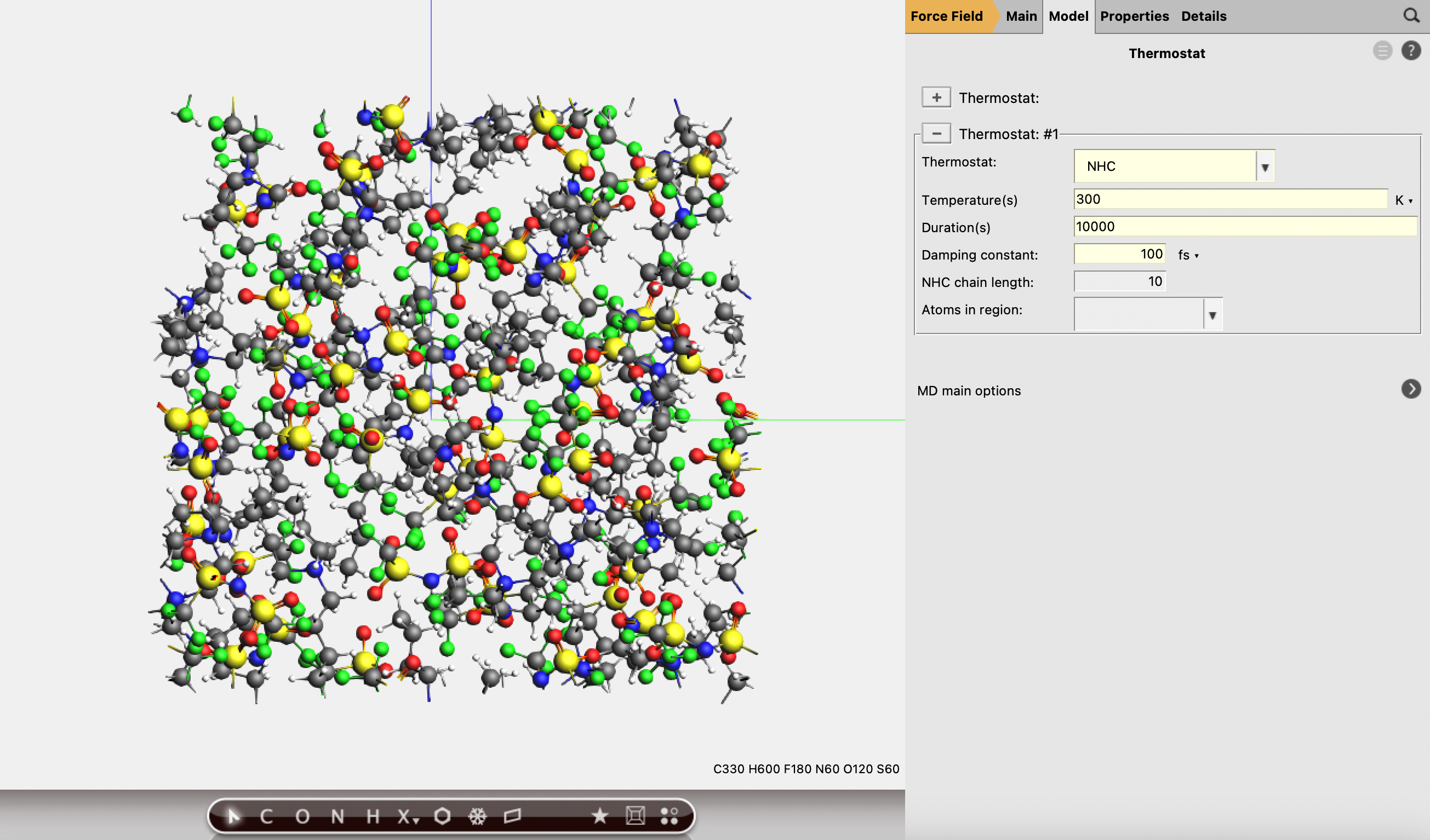
You can now save your input as appViscosity_NVT and run the calculation. Check the box Use MD velocities from result from the pop-up Results found, and click yes to update the coordinates and bonds.
We can now equilibrate the simulation box under isothermal-isobaric conditions (NPT ensemble).
job = AMSNPTJob.restart_from(
    job,
    name="NPT_eq",
    nsteps=10000,
    timestep=0.5,
    samplingfreq=100,
    thermostat="NHC",
    temperature=333,
    tau=100,
    barostat="MTK",
    barostat_tau=1000,
    equal='XYZ',
    writebonds=True,
    writevelocities=False,
    writemolecules=False,
)

Save the input as appViscosity_NPT and run the calculation.
Click SCM → Movie to analyze the last NPT run. Let’s vizualize the density with Graph → Add Graph, followed by MD Properties → Density. Ideally one would want to pursue the NPT equilibration to confirm that the density has converged. We found densities between 1336 and 1346 kg/m3 approximately 2% smaller than the experimental density of 1367 kg/m3.
To reduce the stress on the simulation box we will now select a frame with a small pressure. We first add the pressure to the graph with MD Properties → Pressure and select a frame where the pressure is close to zero. Here you also want to select a late frame in order to insure that the system is equilibrated. You can use the horizontal slide bar to adjust the frame selection. Once the cursor is on a frame with small pressure, click File → Update Geometry In Input. We are now ready to perform the production run.
Production run
For the production run we will perform an NVT simulation as follow:
Note
The last binlog option will write the pressure tensor at every step of the simulation.
job = AMSNVTJob.restart_from(
    job,
    settings=s,
    name="prod",
    nsteps=400000,
    samplingfreq=1000,
    timestep=0.5,
    calcpressure=True,
    binlog_time=True,
    binlog_pressuretensor=True,
    writevelocities=False,
    writemolecules=False,
    writebonds=False
)
Note
Here the binlog command will save the pressure tensor at every step of the simulation, to insure an accurate determination of the viscosity.
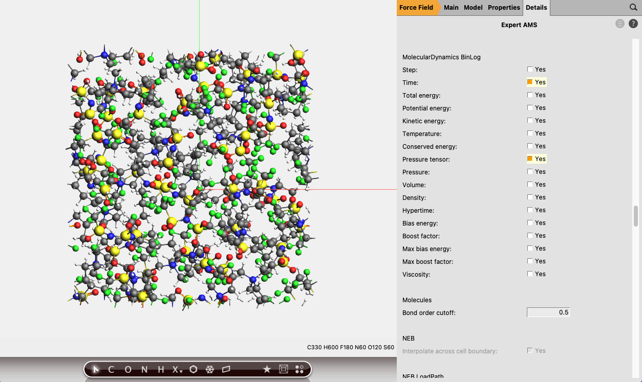
Save the input as appViscosity_prod and run the calculation. You can follow the simulation with SCM → Movie and verify that the initial pressure was close to zero. It can be useful to perform a moving average over the pressure plot to better appreciate the averaged value. To achieve this click Graph → Analysis…, select the Moving Average tab and click the + button below. Here you can modify the window size, for example, 20 steps, and click the OK button.
Note
In order to obtain a converged value of the viscosity the production run should be extended to several nanoseconds.
Computing viscosity
The viscosity of the electrolyte can be calculated using the Green-Kubo relation:
where \(\eta\) is the viscosity, \(V\) is the cell volume, \(k_{\rm{B}}\) is the Boltzmann constant, \(T\) is the temperature, \(P_{\alpha\beta}\) is an off-diagonal component of the pressure tensor, and \(t\) is time. The function \(\langle P_{\alpha\beta}(0)P_{\alpha\beta}(t) \rangle\) is an autocorrelation function with the average taken over all time origins and off-diagonal components (αβ is yz, xz, or xy).
The following Python script will read the pressure tensor from binlog and compute the viscosity from the integral of the off-diagonal pressure tensor autocorrelation function. The resulting viscosity value is interpreted as the limiting value A of a double exponential fit defined as:
#!/usr/bin/env amspython
"""
Usage:
$AMSBIN/amspython viscosity_extractor.py /path/to/ams.rkf

Feel free to change the max_dt_fs to change the maximum correlation time!

The script will produce a file green_kubo_viscosity.txt and viscosity.pdf in the same directory as ams.rkf.
"""

from scm.plams import *
import numpy as np
from scipy.optimize import curve_fit
import matplotlib.pyplot as plt
import os
import sys

def main():
    if len(sys.argv) > 1:
        path_to_rkf = sys.argv[1]
    else:
        path_to_rkf = 'ams.rkf'

    assert os.path.exists(path_to_rkf), f'{path_to_rkf} does not seem to exist. It should be an ams.rkf file.'
    max_dt_fs = 100000
    outfile = os.path.join(os.path.dirname(os.path.abspath(path_to_rkf)), "green_kubo_viscosity.txt")
    compute_pressure_tensor_acf(path_to_rkf, outfile=outfile, max_dt_fs=max_dt_fs)

    assert os.path.exists(outfile), f"{outfile} does not seem to exist!"
    imagefile = os.path.join(os.path.dirname(outfile), "viscosity.pdf")
    viscosity = do_fit(outfile, imagefile=imagefile)

    print(f"Final viscosity: {viscosity:.3f} mPa s")

# The double exponential function
def viscosity_double_exponential(x, A, lam, tau1, tau2):
    return A*( lam*(1-np.exp(-x/tau1)) + (1-lam)*(1-np.exp(-x/tau2)) )

# The main function
def compute_pressure_tensor_acf(path_to_rkf, outfile, max_dt_fs = 100000, discard_first_fs=0):

    # Change this to the path of your ams.rkf file
    job = AMSJob.load_external(path_to_rkf)

    print(f"Computing viscosity for {path_to_rkf}")
    print("Note: this may take several hours if the trajectory is long!")

    # Here we get the off-diagonal pressure tensor from binlog
    xy = job.results.get_history_property('PressureTensor_xy', history_section='BinLog')
    xz = job.results.get_history_property('PressureTensor_xz', history_section='BinLog')
    yz = job.results.get_history_property('PressureTensor_yz', history_section='BinLog')

    minN = min(len(xy), len(xz), len(yz))
    pressuretensor = np.stack( (np.zeros(minN), np.zeros(minN), np.zeros(minN), yz[:minN], xz[:minN], xy[:minN] ), axis=1 )


    # Volume, temperature, time
    volume = job.results.get_main_molecule().unit_cell_volume()
    temperature = np.mean(job.results.get_history_property('Temperature', history_section='MDHistory'))
    times = job.results.get_history_property('Time', history_section='BinLog')
    timestep = times[1]-times[0]

    # We skip first 10000 frames
    discard_first_frames = int(discard_first_fs / timestep)
    pressuretensor = pressuretensor[discard_first_frames:, :]

    # Time interval to compute the ACF
    # We found that max_dt_fs = 100000 fs is a good value
    max_dt = int(max_dt_fs  / timestep)

    # Some info to print
    print(f'Averaged temperature: {temperature}')
    print(f'Timestep: {timestep}')
    print(f'Total simulation time: {times[-1]} fs')
    print(f'Total #frames: {minN}')
    print(f'Discarding first {discard_first_fs:.2f} fs as equilibration period')
    print(f'Discarding first {discard_first_frames} frames as equilibration period')
    print(f'Maximum correlation time: {max_dt_fs:.2f} fs')
    print(f'Maximum correlation time: {max_dt} frames')
    print(f'Unit cell volume: {volume:.3f} ang^3')

    print(f"Calculating the pressure tensor autocorrelation function (this may take a while....)")

    # Compute the viscosity based on GK relation
    x, y = AMSResults._get_green_kubo_viscosity(
        pressuretensor=pressuretensor,
        max_dt=max_dt,
        time_step=timestep,
        volume=volume,
        temperature=temperature
    )

    # We save the data
    print(f"Writing cumulative integral of pressure tensor autocorrelation function to {outfile}")
    A = np.stack((x, y), axis=1)
    np.savetxt(outfile, A, header="Time(fs) Viscosity(mPa*s)")

def do_fit(fname, imagefile):
    A = np.loadtxt(fname)
    x = A[:, 0]
    y = A[:, 1]

    # The fit
    f, p0 = viscosity_double_exponential, (20.0, 0.5, 1000, 10000)
    popt, _ = curve_fit(f, x, y, p0=p0)
    prediction = f(x, *popt)

    # We plot the results
    plt.title(f"Limiting value: {popt[0]:.2f} mPa s")
    plt.plot(x, y, color='tab:blue')
    plt.plot(x, prediction, color='tab:red')
    plt.xlabel("Correlation Time (fs)")
    plt.ylabel("η (mPa s)")
    plt.savefig(imagefile)
    plt.show()

    return popt[0]

if __name__ == '__main__':
    main()
Practically, to extract the viscosity, download the viscosity extractor script, modify the path to your ams.rkf file (corresponding to your production run). You can then run the script with the following command (read more about Python scripting):
$AMSBIN/amspython viscosity_extractor.py /path/to/ams.rkf
Note
If the production simulation is several nanoseconds long, the execution of the Python script can take up to few hours. Indeed, the evaluation of the auto-correlation function over millions of frames is time consuming.
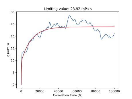
Based on the 400 ps production simulation we obtain a limiting value of \(\eta\) = 23.92 mPa s. Note that although this simulation is short, we obtain a good agreement with the experimental viscosity of the mixture equal to 21.0 mPa s (at 333 K, see Borodin 2009). However, the fluctuations of the viscosity suggest the simulation is not well converged.
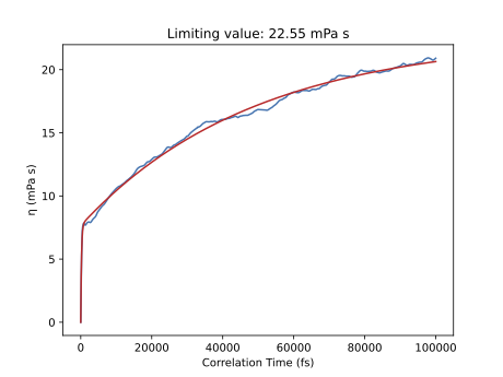
If we continue the previous simulation up to 5 ns, we obtain a limiting value of \(\eta\) = 22.55 mPa s. Here we can well appreciate the convergence of the viscosity, reaching a plateau.
Important considerations
To conclude, we would like to summarize a few general important points in order to achieve quantitative predictions of the viscosity:
The simulation needs to be well equilibrated. Here we started at low density and we deformed the simulation box to target the experimental density. Alternatively, it is possible to gently anneal the system.
In general, make sure to equilibrate the density of the liquid first using an NPT simulation. Verify that the pressure is close to the target value. Then run the NVT production simulation as above.
The viscosity is often sensitive to the supercell size. Use a larger supercell with more molecules for a better value.
The viscosity curve should be smoothly increasing for the entire correlation time.
If the viscosity curve is noisy, decrease the maximum correlation time or run a longer MD simulation. The fitted double exponential should not greatly deviate from the viscosity curve at any point.
Make sure that the simulation is at least 20x longer than the maximum correlation time (but preferably closer to at least 50x longer). Example: if the MD simulation is 2 ns long, set the maximum correlation time in the postanalysis script to (2 ns / 20) = 100 ps or shorter. In the above figure, that maximum correlation time was too long (400 ps simulation / 100 ps maximum correlation time = 4 < 20), as also indicated by the great amount of noise.
The biggest contribution to the integral comes at short correlation times. It is therefore necessary use the BinLog feature, which writes the pressure tensor at every time step.


