Viscosity: Green-Kubo relation
This tutorial will show how to calculate the viscosity of liquid benzene using the Green-Kubo relation:
where \(\eta\) is the viscosity, \(V\) is the cell volume, \(k_{\rm{B}}\) is the Boltzmann constant, \(T\) is the temperature, \(P_{\alpha\beta}\) is an off-diagonal component of the pressure tensor, and \(t\) is time. The function \(<P_{\alpha\beta}(0)P_{\alpha\beta}(t)>\) is an autocorrelation function with the average taken over all time origins and off-diagonal components (αβ is yz, xz, or xy).
The pressure tensor equals the stress tensor plus a kinetic contribution. This tutorial was also featured in our video tip of the week series
Step 1: Create a box of benzene
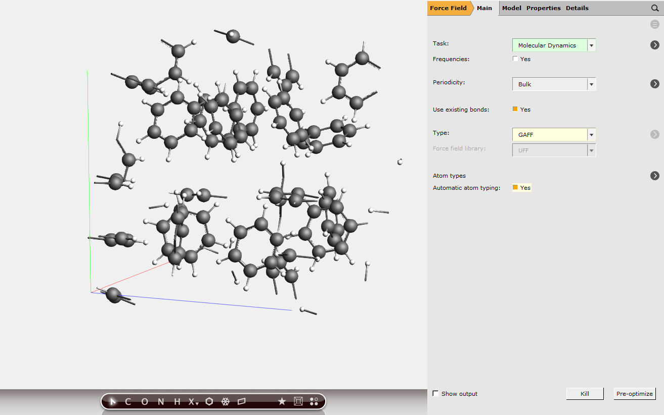
Create a box of 16 benzene molecules with density 0.875 g cm-3
(experimental room-temperature density of benzene) using the Builder in AMSinput,
or download and import a premade xyz file.
13.333 on the diagonal to change the box to a cube of 2370.2 Å3benzene and then click the Benzene (ADF) entry in the list that pops upThe molecules are generated at random positions and orientations, with constraint that all atoms (between different molecules) are at least the specified distance (2.5 Å) apart.

Step 2: Set up the benzene MD simulation
The next step is to set up the details of the simulation.

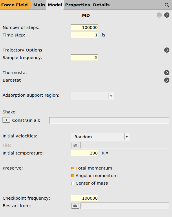
For the MD simulation, we will set up a room-temperature simulation thermostatted with a Nose-Hoover thermostat. It is important to set Sample frequency to a small number. It will save not only the atomic coordinates but also the pressure tensor at that sample frequency, and the pressure tensor needs to be saved frequently to calculate the integral accurately.
1000001 fs5 (or smaller)298 K
NHC298100 fs
We must also tell the AMS driver to calculate the pressure (if you use a barostat, that will happen automatically). To save disk space, we can also turn off most of the things usually saved to the trajectory file, e.g. velocities and molecular bonds, as well as the engine checkpoint files.
100000
Step 3: Run the simulation
Now we will run your set-up:
BenzeneImportant
Double-check that the pressure is calculated. At the start of the simulation, open the logfile (SCM → Logfile), and make sure that numerical values (and not “n/a”) is printed for the pressure. If there is no pressure, then stop the simulation and go back to Step 2.
Note
Running this calculation takes approximately 20 minutes.
Step 4: Analyze the simulation results
Wait until the calculation has finished, and then open it in AMSmovie.
The pressure tensor autocorrelation function should only be calculated after the simulation has equilibrated.
The simulation seems to equilibrated quite quickly. After frame 4000 (time 20 ps) the potential energy seems to fluctuate around a constant value, indicating that the simulation as likely equilibrated at that point.
Frame 4000 corresponds to 20 ps because the time step was 1 fs and the sample frequency 5: 4000*5*1 fs = 20000 fs = 20 ps.
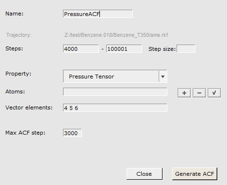
1 to 4000 (this will discard the first 20 ps of the simulation)4 5 6 (these are the off-diagonal elements \(P_{yz}\), \(P_{xz}\), and \(P_{xy}\))3000 (corresponding to a maximum correlation time of 15 ps)

This brings up several graphs in AMSmovie. The bottom graph contains the integral of the pressure tensor autocorrelation function as a function of upper integrand limit:
In the ideal case this graph will converge to a constant value as t → \(\infty\). This usually requires very long simulations. Your graph may look different.
In this case, the integral seems to converge to a value of 1.03 × 10⁻⁹ hartree2 fs bohr-6.
To calculate the viscosity, we also need the volume \(V = 13.333^3 = 2370\) Å3.
Converting everything to SI units (where 1 hartree bohr-3 = 2.942 × 10¹³ Pa), we get
The experimental room-temperature viscosity of benzene is about 0.5 mPa s.
Important considerations
The simulation needs to be well equilibrated
The viscosity is often sensitive to the supercell size. Use a larger supercell with more benzene molecules for a better value.
The integral must converge in the long time-limit. You may want to increase the maximum correlation time (above given as 3000 frames or 15 ps) to a larger value, and increase the simulation time.
The biggest contribution to the integral comes at short correlation times. It is therefore necessary set the Sample frequency to a small number, ideally even smaller than the 5 fs we used here.
In general, make sure to equilibrate the density of the liquid first using an NPT simulation, before running an NVT simulation as above. (the above example used the experimental density, but that may not be suitable for the used force field)
Better and more reliable viscosity values can most likely be obtained using the APPLE&P or GFNFF force fields.
Python script
Both the MD simulation and the calculation of the autocorrelation function (ACF) integral can be scripted with our PLAMS scripting framework. However, extracting the converged viscosity value can be difficult to do automatically. We therefore recommend you to read off the value manually (and not simply use the output from the script).
viscosity.pyand the xyz files for250 K,300 K,350 K.
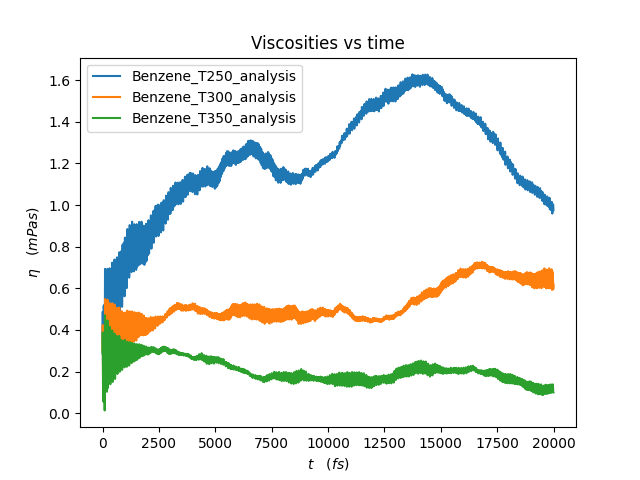
The three xyz-files each contain 16 benzene molecules whose lattice constants have been equilibrated at 250, 300 and 350 K. The script can be run as is and will perform 3 MD runs followed by an analysis. It also provides a method to plot the viscosities so that you are able to read off the converged value yourself, however the script also tries to automatically guess the converged value. It is recommended however to read them off yourself.
Example output:
[18.02|13:41:55] PLAMS working folder: /home/hordijk/Viscosity/Benzene
Beginning viscosity calculations Benzene
I will perform 3 MD runs
Starting MD runs ...
[18.02|13:41:55] JOB Benzene_T250 STARTED
[18.02|13:41:55] JOB Benzene_T300 STARTED
[18.02|13:41:55] JOB Benzene_T350 STARTED
[18.02|13:41:55] Waiting for job Benzene_T250 to finish
[18.02|13:41:55] JOB Benzene_T250 RUNNING
[18.02|13:41:56] JOB Benzene_T300 RUNNING
[18.02|13:41:56] JOB Benzene_T350 RUNNING
[18.02|14:21:18] JOB Benzene_T300 FINISHED
[18.02|14:21:40] JOB Benzene_T300 SUCCESSFUL
[18.02|15:02:37] JOB Benzene_T250 FINISHED
[18.02|15:03:00] JOB Benzene_T250 SUCCESSFUL
[18.02|15:03:00] Waiting for job Benzene_T350 to finish
[18.02|15:42:53] JOB Benzene_T350 FINISHED
[18.02|15:43:04] JOB Benzene_T350 SUCCESSFUL
Starting analysis runs ...
[18.02|15:43:11] JOB Benzene_T250_analysis STARTED
[18.02|15:43:11] JOB Benzene_T300_analysis STARTED
[18.02|15:43:11] JOB Benzene_T350_analysis STARTED
[18.02|15:43:11] Waiting for job Benzene_T250_analysis to finish
[18.02|15:43:11] JOB Benzene_T250_analysis RUNNING
[18.02|15:43:11] JOB Benzene_T300_analysis RUNNING
[18.02|15:43:11] JOB Benzene_T350_analysis RUNNING
[18.02|15:43:24] JOB Benzene_T250_analysis FINISHED
[18.02|15:43:24] JOB Benzene_T350_analysis FINISHED
[18.02|15:43:24] JOB Benzene_T300_analysis FINISHED
[18.02|15:43:24] JOB Benzene_T250_analysis SUCCESSFUL
[18.02|15:43:24] JOB Benzene_T350_analysis SUCCESSFUL
[18.02|15:43:24] JOB Benzene_T300_analysis SUCCESSFUL
[18.02|15:43:25] PLAMS run finished. Goodbye
All calculations are now done
Temperature +- SD (K) | Viscosity (mPa s)
   249.59 +- 14.74  | 1.47419
   300.49 +- 18.50  | 0.47794
   349.92 +- 21.23  | 0.17027

Important
These integrals are not converged, and reading off the viscosities from these plots is unreliable! To get more reliable results, run longer simulations and set SamplingFreq to a smaller number.


